Wie beschrifte ich einen Plot?

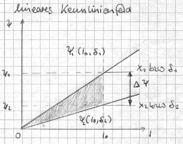
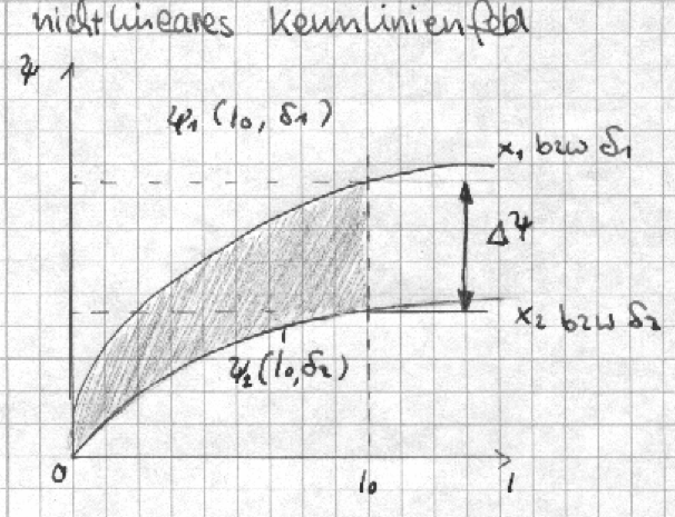
Hallo,

ich habe hier zwei Kennlinienfelder die wie in den Abbildungen beschriftet werden sollen, wie geht das?

Kennlinienfeld 1:

Code, hier editierbar zum Übersetzen:

1
2
3
4
5
6
7
8
9
10
11
12
13
14
15
16
17
18
19
20
21
22
23
24
25
26
27
28
29
30
31
32
33
34
35
36
37
38
39
\documentclass[border=10pt]{standalone}
\usepackage{pgfplots}
\pgfplotsset{compat=1.10}
\usepgfplotslibrary{fillbetween}
\usetikzlibrary{intersections}
\begin{document}
      \begin{tikzpicture}[
        hilfslinie/.style = {help lines, dashed},
        funktion/.style = {black, thick, mark = none}
      ]
      \begin{axis}[
          axis y line = left,
          axis x line = bottom,
          xtick       = \empty,
          ytick       = \empty,
          samples     = 160,
          domain      = 0:5,
          xmax = 6,
          ymax = 6,
          xlabel=$I$,
          ylabel=$\Psi$
        ]
        \addplot[funktion, name path global = funktion1] {0.5*x};
        \addplot[funktion, name path global = funktion2] {1*x};
        \addplot[gray!60] fill between [
          of = funktion1 and funktion2,
          soft clip = {domain = 0:3}
        ] ;
        \path[name path = linie] (axis cs:3,0) -- (axis cs:3,4);
        \draw[hilfslinie, name intersections = {of = funktion1 and linie}]
          ({axis cs:3,0}-|intersection-1) -- (intersection-1);
        \draw[hilfslinie, name intersections = {of = funktion1 and linie}]
          ({axis cs:0,0}|-intersection-1) -- (intersection-1);
        \draw[hilfslinie, name intersections = {of = funktion2 and linie}]
          ({axis cs:0,0}|-intersection-1) -- (intersection-1);
      \end{axis}
    \end{tikzpicture}
\end{document}
 
 
הההההההההההההההההההההההההההההההההההההההההההההההההההההההההההההההההההההההההההההההההההההההההההההההההההההההההההההההההההההההההההההההההההההההההההההההההההההההההההההההההההההההההההההההההההההההההההההההההההההההההההההההההההההההההההההההההההההההההההההההההההההההההההההההה
XXXXXXXXXXXXXXXXXXXXXXXXXXXXXXXXXXXXXXXXXXXXXXXXXXXXXXXXXXXXXXXXXXXXXXXXXXXXXXXXXXXXXXXXXXXXXXXXXXXXXXXXXXXXXXXXXXXXXXXXXXXXXXXXXXXXXXXXXXXXXXXXXXXXXXXXXXXXXXXXXXXXXXXXXXXXXXXXXXXXXXXXXXXXXXXXXXXXXXXXXXXXXXXXXXXXXXXXXXXXXXXXXXXXXXXXXXXXXXXXXXXXXXXXXXXXXXXX

Kennlinienfeld 2:

Open in writeLaTeX

Code, hier editierbar zum Übersetzen:

1
2
3
4
5
6
7
8
9
10
11
12
13
14
15
16
17
18
19
20
21
22
23
24
25
26
27
28
29
30
31
32
33
34
35
36
37
38
\documentclass[border=10pt]{standalone}
\usepackage{pgfplots}
\pgfplotsset{compat=1.10}
\usepgfplotslibrary{fillbetween}
\usetikzlibrary{intersections}
\begin{document}
    \begin{tikzpicture}[
        hilfslinie/.style = {help lines, dashed},
        funktion/.style = {black, thick, mark = none}
      ]
      \begin{axis}[
          axis y line = left,
          axis x line = bottom,
          xtick       = \empty,
          ytick       = \empty,
          samples     = 160,
          domain      = 0:5,
          xmax = 6,
          ymax = 6,
          xlabel=$I$,
          ylabel=$\Psi$
        ]
        \addplot[funktion, name path global = funktion1] {sqrt(x)};
        \addplot[funktion, name path global = funktion2] {2*sqrt(x)};
        \addplot[gray!60] fill between [
          of = funktion1 and funktion2,
          soft clip = {domain = 0:3}
        ] ;
        \path[name path = linie] (axis cs:3,0) -- (axis cs:3,4);
        \draw[hilfslinie, name intersections = {of = funktion1 and linie}]
          ({axis cs:3,0}-|intersection-1) -- (intersection-1);
        \draw[hilfslinie, name intersections = {of = funktion1 and linie}]
          ({axis cs:0,0}|-intersection-1) -- (intersection-1);
        \draw[hilfslinie, name intersections = {of = funktion2 and linie}]
          ({axis cs:0,0}|-intersection-1) -- (intersection-1);
      \end{axis}
    \end{tikzpicture}
\end{document}
 
 
הההההההההההההההההההההההההההההההההההההההההההההההההההההההההההההההההההההההההההההההההההההההההההההההההההההההההההההההההההההההההההההההההההההההההההההההההההההההההההההההההההההההההההההההההההההההההההההההההההההההההההההההההההההההההההההההההההההההההההההההההההההההההההההההה
XXXXXXXXXXXXXXXXXXXXXXXXXXXXXXXXXXXXXXXXXXXXXXXXXXXXXXXXXXXXXXXXXXXXXXXXXXXXXXXXXXXXXXXXXXXXXXXXXXXXXXXXXXXXXXXXXXXXXXXXXXXXXXXXXXXXXXXXXXXXXXXXXXXXXXXXXXXXXXXXXXXXXXXXXXXXXXXXXXXXXXXXXXXXXXXXXXXXXXXXXXXXXXXXXXXXXXXXXXXXXXXXXXXXXXXXXXXXXXXXXXXXXXXXXXXXXXXX

Abbildungen:

alt text

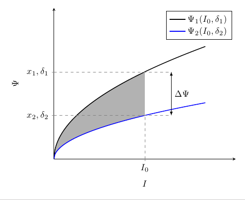
Ich habe hier, wenn auch nicht sehr elegant, mal einen Versuch gestartet:

Open in writeLaTeX

Code, hier editierbar zum Übersetzen:

1
2
3
4
5
6
7
8
9
10
11
12
13
14
15
16
17
18
19
20
21
22
23
24
25
26
27
28
29
30
31
32
33
34
35
36
37
38
39
40
41
\documentclass[border=10pt]{standalone}
\usepackage{pgfplots}
\pgfplotsset{compat=1.10}
\usepgfplotslibrary{fillbetween}
\usetikzlibrary{intersections}
\begin{document}
\begin{tikzpicture}[
    hilfslinie/.style = {help lines, dashed},
    funktion/.style = {black, thick, mark = none}
  ]
  \begin{axis}[
      axis y line = left,
      axis x line = bottom,
      xtick       = \empty,
      ytick       = \empty,
      samples     = 160,
      domain      = 0:5,
      xmax = 6,
      ymax = 6,
      xlabel=$I$,
      ylabel=$\Psi$,
      extra x ticks = {3},
      extra x tick labels = {$I_0$},
      extra y ticks = {3.46475,1.7325},
      extra y tick labels = {${x_1,\delta_1}$, ${x_2,\delta_2}$}
    ]
    \addplot[funktion, name path global = funktion2,color=black] {2*sqrt(x)};
    \addlegendentry{Case 1}
    \addplot[funktion, name path global = funktion1,color=blue] {sqrt(x)};
    \addlegendentry{Case 2}
    \addplot[gray!60] fill between [
      of = funktion1 and funktion2,
      soft clip = {domain = 0:3}
    ] ;
    \path[name path = linie] (axis cs:3,0) -- (axis cs:3,4);
    \draw[hilfslinie, name intersections = {of = funktion1 and linie}]
      ({axis cs:3,0}-|intersection-1) -- (intersection-1);
    \draw[hilfslinie, name intersections = {of = funktion1 and linie}]
      ({axis cs:0,0}|-intersection-1) -- (intersection-1);
    \draw[hilfslinie, name intersections = {of = funktion2 and linie}]
 
 
הההההההההההההההההההההההההההההההההההההההההההההההההההההההההההההההההההההההההההההההההההההההההההההההההההההההההההההההההההההההההההההההההההההההההההההההההההההההההההההההההההההההההההההההההההההההההההההההההההההההההההההההההההההההההההההההההההההההההההההההההההההההההההההההה
XXXXXXXXXXXXXXXXXXXXXXXXXXXXXXXXXXXXXXXXXXXXXXXXXXXXXXXXXXXXXXXXXXXXXXXXXXXXXXXXXXXXXXXXXXXXXXXXXXXXXXXXXXXXXXXXXXXXXXXXXXXXXXXXXXXXXXXXXXXXXXXXXXXXXXXXXXXXXXXXXXXXXXXXXXXXXXXXXXXXXXXXXXXXXXXXXXXXXXXXXXXXXXXXXXXXXXXXXXXXXXXXXXXXXXXXXXXXXXXXXXXXXXXXXXXXXXXX

Leider bekomme ich diese Delta Psi Bemaßung zwischen den Kurven nicht hin. Desweiteren gibt es sicher eine bessere Variante für die y-Beschriftung, als die Punkte so genau zu suchen (3.46475,1.7325).

beschriftungen pgfplots

gefragt 09 Jun '14, 09:51

Patrick1990
114●4●7●11
Akzeptiert-Rate: 0%

bearbeitet 09 Jun '14, 11:13

Eine Antwort:

active answers älteste Antworten neueste Antworten Beliebteste Antworten

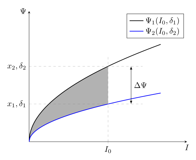
Hier ist mal noch eine Alternative ohne zusätzliche Bibliotheken. Für die Beschriftung der y-Achse werden die Schnittpunkte der Hilfslinien mit dieser verwendet, weshalb keine separate Berechnung notwendig ist. Die Label für die Achsen habe ich zu den Pfeilspitzen verschoben.

Open in writeLaTeX

Code, hier editierbar zum Übersetzen:

1
2
3
4
5
6
7
8
9
10
11
12
13
14
15
16
17
18
19
20
21
22
23
24
25
26
27
28
29
30
31
32
33
34
35
36
37
38
39
40
41
\documentclass[border=10pt]{standalone}
\usepackage{pgfplots}
\pgfplotsset{compat=1.10}
\usepgfplotslibrary{fillbetween}
\usetikzlibrary{intersections}
\begin{document}
\begin{tikzpicture}[
    hilfslinie/.style = {help lines, dashed},
    differenz/.style = {latex-latex,thin},
    funktion/.style = {black, thick, mark = none}
  ]
  \begin{axis}[
      axis y line = left,
      axis x line = bottom,
      xtick       = \empty,
      ytick       = \empty,
      samples     = 160,
      domain      = 0:5,
      xmax = 6,
      ymax = 6,
      xtick=3,
      xticklabels={$I_0$},
      xlabel=$I$,
      xlabel style={at={(rel axis cs:1,0)}},
      ylabel=$\Psi$,
      ylabel style={at={(rel axis cs:0,1)},rotate=-90},
    ]
    \addplot[funktion, name path global = funktion2,color=black] {2*sqrt(x)};
    \addlegendentry{Case 1}
    \addplot[funktion, name path global = funktion1,color=blue] {sqrt(x)};
    \addlegendentry{Case 2}
    \addplot[gray!60] fill between [
      of = funktion1 and funktion2,
      soft clip = {domain = 0:3}
    ] ;
    \path[name path = linie] (axis cs:3,0) -- (axis cs:3,4);
    \path[name intersections = {of = funktion1 and linie,by=p1}];
    \path[name intersections = {of = funktion2 and linie,by=p2}];
    \draw[hilfslinie]
      ({axis cs:0,0}|-p1)coordinate(yl1)--([xshift=1.5cm]p1)
 
 
הההההההההההההההההההההההההההההההההההההההההההההההההההההההההההההההההההההההההההההההההההההההההההההההההההההההההההההההההההההההההההההההההההההההההההההההההההההההההההההההההההההההההההההההההההההההההההההההההההההההההההההההההההההההההההההההההההההההההההההההההההההההההההההההה
XXXXXXXXXXXXXXXXXXXXXXXXXXXXXXXXXXXXXXXXXXXXXXXXXXXXXXXXXXXXXXXXXXXXXXXXXXXXXXXXXXXXXXXXXXXXXXXXXXXXXXXXXXXXXXXXXXXXXXXXXXXXXXXXXXXXXXXXXXXXXXXXXXXXXXXXXXXXXXXXXXXXXXXXXXXXXXXXXXXXXXXXXXXXXXXXXXXXXXXXXXXXXXXXXXXXXXXXXXXXXXXXXXXXXXXXXXXXXXXXXXXXXXXXXXXXXXXX

alt text

Permanenter link

beantwortet 09 Jun '14, 13:47

esdd
17.8k●30●42●57
Akzeptiert-Rate: 62%

bearbeitet 12 Jun '14, 08:50

Hier ein Vorschlag für die Beschriftung der Differenz.

Ich lade die positioning library, die man eh öfter mal gebrauchen kann (für die right of Syntax), und bestimme Koordinaten delta1 und delta2 jeweils rechts vom Schnitt. Die Hilfslinien zeichne ich dann gleich durch.

Den Beschriftungspfeil mit beidseitiger Spitze zeichne ich als edge mit node als Beschriftung.

Open in writeLaTeX

Code, hier editierbar zum Übersetzen:

1
2
3
4
5
6
7
8
9
10
11
12
13
14
15
16
17
18
19
20
21
22
23
24
25
26
27
28
29
30
31
32
33
34
35
36
37
38
39
40
41
\documentclass[border=10pt]{standalone}
\usepackage{pgfplots}
\pgfplotsset{compat=1.10}
\usepgfplotslibrary{fillbetween}
\usetikzlibrary{intersections,positioning,arrows}
\begin{document}
\begin{tikzpicture}[
    hilfslinie/.style = {help lines, dashed},
    funktion/.style = {black, thick, mark = none}
  ]
  \begin{axis}[
      axis y line = left,
      axis x line = bottom,
      xtick       = \empty,
      ytick       = \empty,
      samples     = 160,
      domain      = 0:5,
      xmax = 6,
      ymax = 6,
      xlabel=$I$,
      ylabel=$\Psi$,
      extra x ticks = {3},
      extra x tick labels = {$I_0$},
      extra y ticks = {3.46475,1.7325},
      extra y tick labels = {${x_1,\delta_1}$, ${x_2,\delta_2}$}
    ]
    \addplot[funktion, name path global = funktion2,color=black] {2*sqrt(x)};
    \addlegendentry{Case 1}
    \addplot[funktion, name path global = funktion1,color=blue] {sqrt(x)};
    \addlegendentry{Case 2}
    \addplot[gray!60] fill between [
      of = funktion1 and funktion2,
      soft clip = {domain = 0:3}
    ] ;
    \path[name path = linie] (axis cs:3,0) -- (axis cs:3,4);
    \coordinate [name intersections = {of = funktion1 and linie},
      right of = intersection-1] (delta1);
    \draw[hilfslinie] ({axis cs:3,0}-|intersection-1) -- (intersection-1);
    \draw[hilfslinie] ({axis cs:0,0}|-intersection-1) -- (delta1);
    \coordinate [name intersections = {of = funktion2 and linie},
 
 
הההההההההההההההההההההההההההההההההההההההההההההההההההההההההההההההההההההההההההההההההההההההההההההההההההההההההההההההההההההההההההההההההההההההההההההההההההההההההההההההההההההההההההההההההההההההההההההההההההההההההההההההההההההההההההההההההההההההההההההההההההההההההההההההה
XXXXXXXXXXXXXXXXXXXXXXXXXXXXXXXXXXXXXXXXXXXXXXXXXXXXXXXXXXXXXXXXXXXXXXXXXXXXXXXXXXXXXXXXXXXXXXXXXXXXXXXXXXXXXXXXXXXXXXXXXXXXXXXXXXXXXXXXXXXXXXXXXXXXXXXXXXXXXXXXXXXXXXXXXXXXXXXXXXXXXXXXXXXXXXXXXXXXXXXXXXXXXXXXXXXXXXXXXXXXXXXXXXXXXXXXXXXXXXXXXXXXXXXXXXXXXXXX

Beschriftung

Permanenter link

beantwortet 09 Jun '14, 12:10

stefan ♦♦
18.4k●16●31●48
Akzeptiert-Rate: 50%

Vielen Dank, habe nun alles, was ich brauche. Werde mich mal durchdenken, auf den linearen Plot konnte ich alles übertragen. Gibt es denn noch eine elegantere Lösung für diese y-Beschriftung?

(09 Jun '14, 13:05) Patrick1990

Deine Antwort

[Vorschau ausblenden]

Community Wiki:

Folgen dieser Frage

Per E-Mail:

Wenn sie sich anmelden, kommen Sie für alle Updates hier in Frage

Per RSS:

Antworten

Antworten und Kommentare

Frage-Themen:

pgfplots ×298
beschriftungen ×50

gestellte Frage: 09 Jun '14, 09:51

Frage wurde gesehen: 12,862 Mal

zuletzt geändert: 12 Jun '14, 08:50

Wie beschrifte ich einen Plot?

Folgen dieser Frage

verwandte Fragen